We will use example provided in the official implementation of the KAN paper. Install the library with
pip install pykan
Function Fitting
We will take Example-1 provided in the PyKAN repo.
The function is \[
f(x) = \sin(\pi x_1) + x_2^2 \\
x_1, x_2 \sim U[-1,1]
\]
import torchimport matplotlib.pyplot as plt= torch.device('cuda' if torch.cuda.is_available() else 'cpu' )print ('device is: ' ,device)from kan.utils import create_dataset= lambda x: torch.exp(torch.sin(torch.pi* x[:,[0 ]]) + x[:,[1 ]]** 2 )= create_dataset(f, n_var= 2 , device= device)print ('train input data shape' , dataset['train_input' ].shape)print ('train label data shape' , dataset['train_label' ].shape)
device is:  cpu
train input data shape torch.Size([1000, 2])
train label data shape torch.Size([1000, 1])
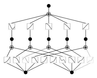
# create a KAN: 2D inputs, 1D output, and 5 hidden neurons. cubic spline (k=3), 5 grid intervals (grid=5). from kan import KAN= KAN(width= [2 ,5 ,1 ], grid= 3 , k= 3 , seed= 42 , device= device)
checkpoint directory created: ./model
saving model version 0.0
# plot KAN at initialization 'train_input' ]);
# train the model = "LBFGS" , steps= 50 , lamb= 0.001 );
| train_loss: 1.88e-02 | test_loss: 1.78e-02 | reg: 6.80e+00 | : 100%|█| 50/50 [00:13<00:00, 3.79it
# visualise the trained model
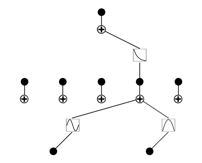
# prune the model, and revisualize = model.prune()
# contnue retraining based on the pruned model = "LBFGS" , steps= 50 );
| train_loss: 1.79e-02 | test_loss: 1.72e-02 | reg: 7.66e+00 | : 100%|█| 50/50 [00:03<00:00, 13.81it
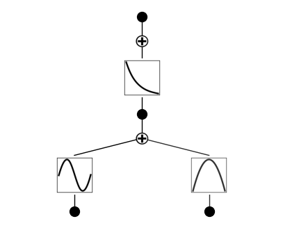
= "auto" # "manual" if mode == "manual" :# manual mode 0 ,0 ,0 ,'sin' ); 0 ,1 ,0 ,'x^2' ); 1 ,0 ,0 ,'exp' ); elif mode == "auto" :# automatic mode = ['x' ,'x^2' ,'x^3' ,'x^4' ,'exp' ,'log' ,'sqrt' ,'tanh' ,'sin' ,'abs' ]= lib)
fixing (0,0,0) with sin, r2=0.9998313640557426, c=2
fixing (0,1,0) with x^2, r2=0.9999907195889106, c=2
fixing (1,0,0) with exp, r2=0.9999810964976568, c=2
saving model version 0.4
# continue retrained and fit the symbolic functions that were found earlier = "LBFGS" , steps= 50 );
| train_loss: 9.43e-12 | test_loss: 5.75e-12 | reg: 0.00e+00 | : 100%|█| 50/50 [00:01<00:00, 27.50it
# plot the symbolic model from kan.utils import ex_round0 ][0 ],4 )
\(\displaystyle 1.0 e^{1.0 x_{2}^{2} + 1.0 \sin{\left(3.1416 x_{1} \right)}}\)
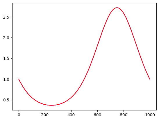
= dataset['train_input' ]= 1000 0 ] = torch.linspace(- 1 ,1 ,steps= n)1 ] = torch.zeros(n)= f(X)= y[:,0 ].detach().numpy()= model.forward(X)= yh[:,0 ].detach().numpy()= 'blue' )= 'red' )
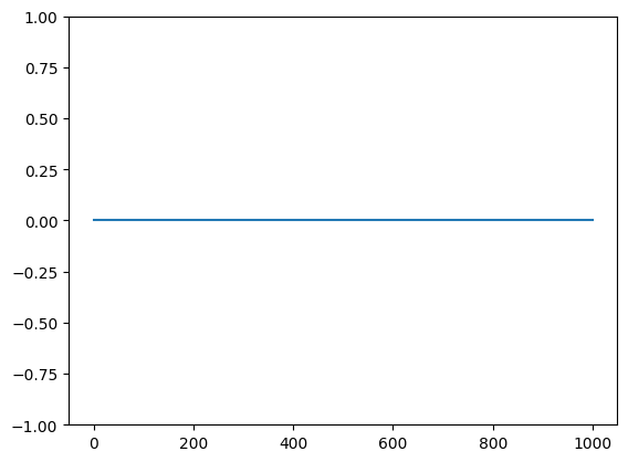
- yh)- 1 ,1 )
Indeed, the correct function was recovered, exactly. This would have been very hard for an MLP. Let us how a off-the-shelf (meaning no tuning) MLP will work out of the box. We will copy an MLP from this regression notebook.
import torch.nn as nn# define the model. # the model is exactly the same as the model we saw in earlier class MLP(nn.Module):# define nn def __init__ (self , input_dim= 4 , output_dim= 3 , hidden_dim = [128 ,64 ]):super (MLP, self ).__init__ ()self .input = nn.Linear(input_dim, hidden_dim[0 ])self .hidden = nn.Linear(hidden_dim[0 ], hidden_dim[1 ])self .out = nn.Linear(hidden_dim[1 ], output_dim)self .relu = nn.ReLU()self .silu = nn.SiLU()def forward(self , X):= self .silu(self .input (X))= self .silu(self .hidden(X))= self .out(X)return X
= 2 = 1 = [64 , 64 ]= MLP(input_dim= input_dim, output_dim= output_dim, hidden_dim= hidden_dim)= 0.01 = nn.MSELoss()= torch.optim.Adam(mlp.parameters(),lr= learning_rate)
def train_network(model,optimizer,criterion,X_train,y_train,X_test,y_test,num_epochs,train_losses,test_losses):for epoch in range (num_epochs):#clear out the gradients from the last step loss.backward() #forward feed = model(X_train)#calculate the loss = criterion(output_train, y_train)#backward propagation: calculate gradients #update the weights eval ()= model(X_test)= criterion(output_test,y_test)= loss_train.item()= loss_test.item()if (epoch + 1 ) % 50 == 0 :print (f"Epoch { epoch+ 1 } / { num_epochs} , Train Loss: { loss_train. item():.4f} , Test Loss: { loss_test. item():.4f} " )return model, train_losses, test_lossesimport numpy as np= 1000 = np.zeros(num_epochs)= np.zeros(num_epochs)= dataset['train_input' ]= dataset['train_label' ]= dataset['test_input' ]= dataset['test_label' ]= train_network(mlp,optimizer,criterion,X_train,y_train,X_test,y_test,num_epochs,train_losses,test_losses)
Epoch 50/1000, Train Loss: 2.0488, Test Loss: 1.8635
Epoch 100/1000, Train Loss: 2.0481, Test Loss: 1.8814
Epoch 150/1000, Train Loss: 2.0478, Test Loss: 1.8812
Epoch 200/1000, Train Loss: 2.0476, Test Loss: 1.8800
Epoch 250/1000, Train Loss: 2.0474, Test Loss: 1.8780
Epoch 300/1000, Train Loss: 2.0468, Test Loss: 1.8737
Epoch 350/1000, Train Loss: 2.0453, Test Loss: 1.8607
Epoch 400/1000, Train Loss: 2.0437, Test Loss: 1.8382
Epoch 450/1000, Train Loss: 2.0425, Test Loss: 1.8111
Epoch 500/1000, Train Loss: 2.0418, Test Loss: 1.7928
Epoch 550/1000, Train Loss: 2.0415, Test Loss: 1.7889
Epoch 600/1000, Train Loss: 2.0413, Test Loss: 1.7895
Epoch 650/1000, Train Loss: 2.0411, Test Loss: 1.7912
Epoch 700/1000, Train Loss: 2.0411, Test Loss: 1.7929
Epoch 750/1000, Train Loss: 2.0410, Test Loss: 1.7938
Epoch 800/1000, Train Loss: 2.0410, Test Loss: 1.7942
Epoch 850/1000, Train Loss: 2.0409, Test Loss: 1.7945
Epoch 900/1000, Train Loss: 2.0408, Test Loss: 1.7956
Epoch 950/1000, Train Loss: 2.0406, Test Loss: 1.7987
Epoch 1000/1000, Train Loss: 2.0403, Test Loss: 1.8046
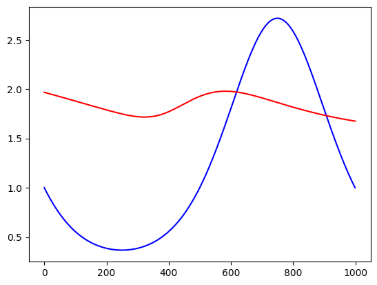
= len (X_train)0 ] = torch.linspace(- 1 ,1 ,steps= n)1 ] = torch.zeros(n)= f(X)= y[:,0 ].detach().numpy()= mlp(X)= yh[:,0 ].detach().numpy()= 'blue' )= 'red' )
The MLP has hard time learning this function. Architectures search and tuning hyperparams is needed.
