A notebook to apply an FFN (Feed Forward Neural Network) to classify the flower species type. We will use the the famous Iris dataset (which is now the equivalent of the hellow world dataset in the Data Science World)
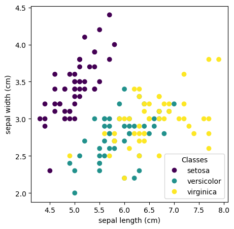
sklearn comes with Iris dataset. We will load it, and do some basic visualization. It is always a good idea to “look” at the data before (blindly) running any models.
We see that, 1. there are four features, and it is a three class classification problem 2. Using two features (sepal length, and sepal width), it is clear that, a perceptron will not be able separate _versicolor from virginica (data is not linearly separable) class. 3. But setosa can be separated from the remaining two.
Let us look at the basic descriptions of the data.
print('feature name',iris.feature_names)print('features type of data',type(iris.data))print('features shape',iris.data.shape)print('feature name',iris.target_names)print('target type of data',type(iris.target))print('target shape',iris.target.shape)
feature name ['sepal length (cm)', 'sepal width (cm)', 'petal length (cm)', 'petal width (cm)']
features type of data <class 'numpy.ndarray'>
features shape (150, 4)
feature name ['setosa' 'versicolor' 'virginica']
target type of data <class 'numpy.ndarray'>
target shape (150,)
Ha. In the original dataset, the data is organized by class. If we naively prepare the mini batches (sequentially), model will only see data corresponding to only one class. This will be pretty problematic to get proper gradient signals. We should shuffle the data s.t diversity in the mini batches is maintained.
Questions
Imagine you split the data into two batches. One containing only say class 0, and other contains only class 1. During training, the model sees these two batches cyclically. Will the model ever converge.
Will it converge when the data is linearly separable?
Will it converge when the data is not linearly separable?
Does having a balanced class representation in every mini batch helps? Which way does it?
What will be the impact of learning rate when alternating between sets of samples of one class during gradient descent?
Let us get back to checking the data, this time, from huggingace datasets itself. Later down the line, it may be useful to learn how to work with datasets library from HuggingFace. It has deep integrations with PyTorch.
from datasets import Datasetimport pandas as pddf = pd.read_csv("hf://datasets/scikit-learn/iris/Iris.csv")df = pd.DataFrame(df)df.head()
Interestingly, the first column is ids., which is not useful for us. May be, a perfect system can simply memory the indices and spit out the correct classes.
And we need to map the Iris types into numerical codes for models to work with. In the torch, we can supply integers representing the classes, and we do not have to explicitly pass one-hot coded labels.
# transform species to numericsdf.loc[df.Species=='Iris-setosa', 'Target'] =0df.loc[df.Species=='Iris-versicolor', 'Target'] =1df.loc[df.Species=='Iris-virginica', 'Target'] =2print(df.Target.unique())df.head()
[0. 1. 2.]
Id
SepalLengthCm
SepalWidthCm
PetalLengthCm
PetalWidthCm
Species
Target
0
1
5.1
3.5
1.4
0.2
Iris-setosa
0.0
1
2
4.9
3.0
1.4
0.2
Iris-setosa
0.0
2
3
4.7
3.2
1.3
0.2
Iris-setosa
0.0
3
4
4.6
3.1
1.5
0.2
Iris-setosa
0.0
4
5
5.0
3.6
1.4
0.2
Iris-setosa
0.0
# drop the Id columns from the dataframedf.drop(['Id'],axis=1,inplace=True)df.head()
Above (visualluy inspecting data) is not a rigorous way (and repeatable way) to test if the data is shuffled (randomly). For numerical labels like integers, in the multi-class or binary class classification problems, which statistical test is suitable to flag if the data grouped?
# scale the features to roughly have zero mean and unit variancefrom sklearn.preprocessing import StandardScalerscaler = StandardScaler()X_train = scaler.fit_transform(X_train)X_test = scaler.transform(X_test)
It is always a good practice to scale the data (features).
What might happen if the different features are on different scales?
Does it pose any problems for the optimizer (gradient descent)?
Does it cause any problems w.r.t interpretation of the feature importance?
Let us define a FFN (or MLP) with two hidden layers. Suppose \(x\) is a \(B \times 4\) vector, we have two hidden layers of 64 dimensions each, and we have three outputs (one for each class), then, \[
h_1 = ReLU(x W_{1} +b_{1}) \\
h_2 = ReLU(h_1 W_{2} +b_{2}) \\
y = h_2 W_{out} + b_{out} \\
\]
where \[
x \text{ is } B \times 4 \\
W_{1} \text{ is } 4 \times 64 \\
W_{2} \text{ is } 64 \times 64 \\
W_{out} \text{ is } 64 \times 3 \\
b_{1} \text{ is } 1 \times 64 \\
b_{2} \text{ is } 1 \times 64 \\
b_{out} \text{ is } 1 \times 3 \\
y \text{ is } B \times 3 \\
\]
In $xW +b $, \(b\) is broadcast over all rows and \(B\) is the batch size.
\(ReLU(x) = x \text{ if } x \ge 0 \text{ and } 0 \text{ o.w }\)
Question
What is the total number of parameters if input dimension is \(p^{in}\), output dimension is \(p^{out}\) and each hidden layer is of size \(p^{h}_{i}\) for the i-th hidden layer and there \(d\) such layers?
class MLP(nn.Module):# define nndef__init__(self, input_dim=4, output_dim=3, hidden_dim = [128,64]):super(MLP, self).__init__()self.h1 = nn.Linear(input_dim, hidden_dim[0])self.h2 = nn.Linear(hidden_dim[0], hidden_dim[1])self.out = nn.Linear(hidden_dim[1], output_dim)self.relu = nn.ReLU()def forward(self, X): X =self.relu(self.h1(X)) X =self.relu(self.h2(X)) X =self.out(X)return X
We have built a Neural Network with one input layer, two hidden layers, and one output layer.
Note, the last output layer is a linear layer. Even though we are modeling a 3-class problem, output layer is still linear, and not softmax. Is this fine?
input_dim =4# No. of featuresoutput_dim =3# No. of outputshidden_dim = [64, 64] # No. of perceptrons in 1st hidden layer and 2nd hidden layermodel = MLP(input_dim=input_dim, output_dim=output_dim, hidden_dim=hidden_dim) # instantiate the model
# inspect the model for a given batch sizefrom torchinfo import summarysummary(model, input_size=(10, 4))
def get_accuracy_multiclass(pred_arr,original_arr):iflen(pred_arr)!=len(original_arr):returnFalse pred_arr = pred_arr.numpy() original_arr = original_arr.numpy() final_pred= []# we will get something like this in the pred_arr [32.1680,12.9350,-58.4877]# so will be taking the index of that argument which has the highest value here 32.1680 which corresponds to 0th indexfor i inrange(len(pred_arr)): final_pred.append(np.argmax(pred_arr[i])) final_pred = np.array(final_pred) count =0#here we are doing a simple comparison between the predicted_arr and the original_arr to get the final accuracyfor i inrange(len(original_arr)):if final_pred[i] == original_arr[i]: count+=1return count/len(final_pred)
Notice that the model predictions were of size (batch_size, output_dim) and we have to take argmax of the model predictions to produce the class labels. The predictions are in the logit space (recall that the output layer is linear and not softmax).