FFNs Regression

A notebook to apply an FFN (Feed Forward Neural Network) to regress. We will use Friedman2 dataset from sklearn

Based on - Kaggle Notebook for Iris Classiifcation - PyTorch for Iris Dataset - Iris Classification

import matplotlib.pyplot as plt

from sklearn.datasets import make_friedman2
X, y = make_friedman2(n_samples = 200, random_state=42, noise=0.5)
print(X.shape)
print(y.shape)

(200, 4)
(200,)

plt.figure(figsize=(5,5))
plt.scatter(X[:,0],y)
plt.show()
plt.hist(y)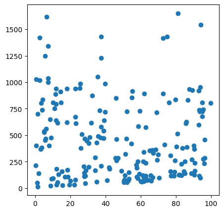

(array([64., 29., 30., 19., 23., 20.,  5.,  2.,  5.,  3.]),
 array([  13.8686335 ,  177.60233879,  341.33604407,  505.06974936,
         668.80345464,  832.53715992,  996.27086521, 1160.00457049,
        1323.73827578, 1487.47198106, 1651.20568635]),
 <BarContainer object of 10 artists>)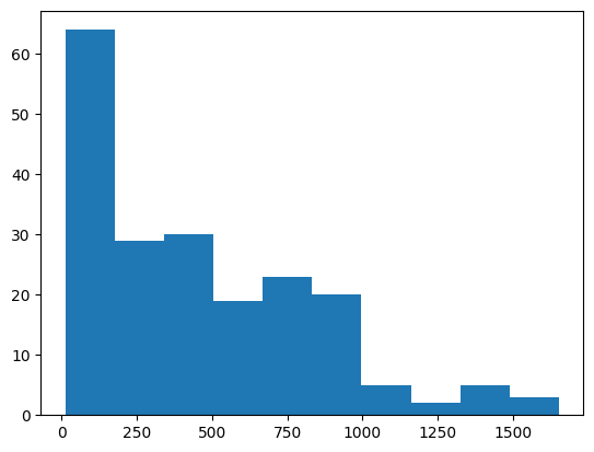

# split and scale.
from sklearn.model_selection import train_test_split
X_train, X_test, y_train, y_test = train_test_split(X,y, test_size=0.2)

from sklearn.preprocessing import StandardScaler

scaler = StandardScaler()
X_train = scaler.fit_transform(X_train)
X_test = scaler.transform(X_test)

# Friedman2 response variable has huge dynamic range. The maximum value seems above above 1500.
scaler = StandardScaler()

print(y_train.shape)
y_tmp = y_train.reshape(-1, 1)
y_train = scaler.fit_transform(y_tmp)
print(y_train.shape)

y_tmp = y_test.reshape(-1, 1)
y_test = scaler.transform(y_tmp)
print(y_test.shape)

(160,)
(160, 1)
(40, 1)

Exercise

Run the regression without scaling the response variable! What will be expected?

# load the libraries
import pandas as pd
from sklearn.model_selection import train_test_split
from sklearn.metrics import accuracy_score, precision_score, recall_score

import torch
import torch.nn as nn
import torch.nn.functional as F
from torch.autograd import Variable

# convert numpy arrays into torch tensors
X_train = torch.FloatTensor(X_train)
X_test = torch.FloatTensor(X_test)
y_train = torch.FloatTensor(y_train)
y_test = torch.FloatTensor(y_test)

# define the model.
# the model is exactly the same as the model we saw in earlier
class MLP(nn.Module):
    # define nn
    def __init__(self, input_dim=4, output_dim=3, hidden_dim = [128,64]):
        super(MLP, self).__init__()
        self.input = nn.Linear(input_dim, hidden_dim[0])
        self.hidden = nn.Linear(hidden_dim[0], hidden_dim[1])
        self.out = nn.Linear(hidden_dim[1], output_dim)
        self.relu = nn.ReLU()

    def forward(self, X):
        X = self.relu(self.input(X))
        X = self.relu(self.hidden(X))
        X = self.out(X)
        return X

input_dim = 4
output_dim = 1
hidden_dim = [64, 64]
model = MLP(input_dim=input_dim, output_dim=output_dim, hidden_dim=hidden_dim)

learning_rate = 0.01
criterion = nn.MSELoss()
optimizer = torch.optim.Adam(model.parameters(),lr=learning_rate)

Since it is a regression problem, we have used MSE loss. Practically, this is the only change we have to make so far. And of course, how to evaluate the model perdictions has to change!

def train_network(model,optimizer,criterion,X_train,y_train,X_test,y_test,num_epochs,train_losses,test_losses):
    for epoch in range(num_epochs):
        #clear out the gradients from the last step loss.backward()
        optimizer.zero_grad()
        
        #forward feed
        output_train = model(X_train)

        #calculate the loss
        loss_train = criterion(output_train, y_train)


        #backward propagation: calculate gradients
        loss_train.backward()

        #update the weights
        optimizer.step()
        
        output_test = model(X_test)
        loss_test = criterion(output_test,y_test)

        train_losses[epoch] = loss_train.item()
        test_losses[epoch] = loss_test.item()

        if (epoch + 1) % 50 == 0:
            print(f"Epoch {epoch+1}/{num_epochs}, Train Loss: {loss_train.item():.4f}, Test Loss: {loss_test.item():.4f}")

import numpy as np
num_epochs = 1000
train_losses = np.zeros(num_epochs)
test_losses  = np.zeros(num_epochs)
train_network(model,optimizer,criterion,X_train,y_train,X_test,y_test,num_epochs,train_losses,test_losses)

Epoch 50/1000, Train Loss: 0.0040, Test Loss: 0.0068
Epoch 100/1000, Train Loss: 0.0010, Test Loss: 0.0037
Epoch 150/1000, Train Loss: 0.0005, Test Loss: 0.0032
Epoch 200/1000, Train Loss: 0.0003, Test Loss: 0.0028
Epoch 250/1000, Train Loss: 0.0002, Test Loss: 0.0026
Epoch 300/1000, Train Loss: 0.0001, Test Loss: 0.0025
Epoch 350/1000, Train Loss: 0.0001, Test Loss: 0.0025
Epoch 400/1000, Train Loss: 0.0001, Test Loss: 0.0024
Epoch 450/1000, Train Loss: 0.0016, Test Loss: 0.0037
Epoch 500/1000, Train Loss: 0.0000, Test Loss: 0.0024
Epoch 550/1000, Train Loss: 0.0000, Test Loss: 0.0023
Epoch 600/1000, Train Loss: 0.0008, Test Loss: 0.0030
Epoch 650/1000, Train Loss: 0.0000, Test Loss: 0.0023
Epoch 700/1000, Train Loss: 0.0000, Test Loss: 0.0022
Epoch 750/1000, Train Loss: 0.0000, Test Loss: 0.0022
Epoch 800/1000, Train Loss: 0.0002, Test Loss: 0.0024
Epoch 850/1000, Train Loss: 0.0000, Test Loss: 0.0022
Epoch 900/1000, Train Loss: 0.0000, Test Loss: 0.0022
Epoch 950/1000, Train Loss: 0.0000, Test Loss: 0.0021
Epoch 1000/1000, Train Loss: 0.0000, Test Loss: 0.0024

plt.figure(figsize=(5,5))
plt.plot(train_losses, label='train loss')
plt.plot(test_losses, label='test loss')
plt.legend()
plt.show()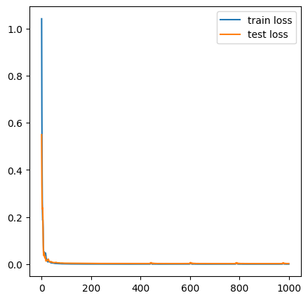

predictions_train = []
predictions_test =  []
with torch.no_grad():
    predictions_train = model(X_train)
    predictions_test = model(X_test)

print(predictions_train.shape)
print(type(predictions_train))

print(y_train.shape)
print(type(y_train))

torch.Size([160, 1])
<class 'torch.Tensor'>
torch.Size([160, 1])
<class 'torch.Tensor'>

yt = y_test.numpy()
print(type(yt))
print(yt.shape)

yh = predictions_test.numpy()
print(type(yh))
print(yh.shape)

<class 'numpy.ndarray'>
(40, 1)
<class 'numpy.ndarray'>
(40, 1)

from sklearn.metrics import mean_squared_error as mse
from sklearn.metrics import root_mean_squared_error as rmse

print('mse is: ', mse(yt, yh))
print('rmse is: ', rmse(yt, yh))

mse is:  0.00236044
rmse is:  0.04858436

plt.scatter(yt,yh)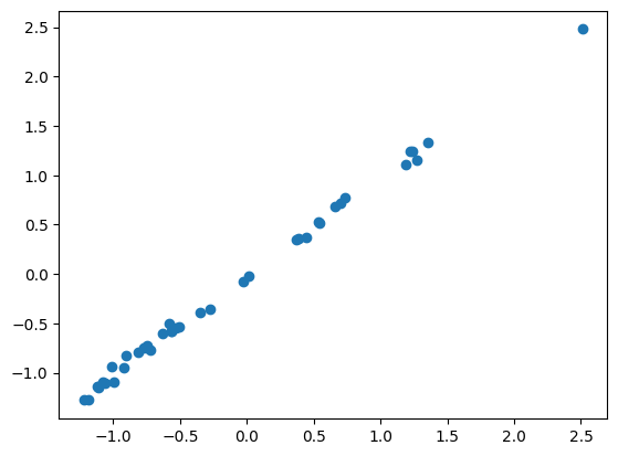

residuals = yt-yh
plt.hist(residuals)
plt.show()

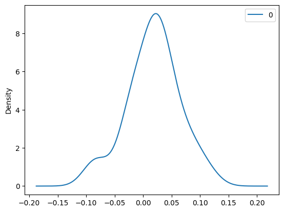
import pandas as pd
pd.DataFrame(residuals).plot(kind='density')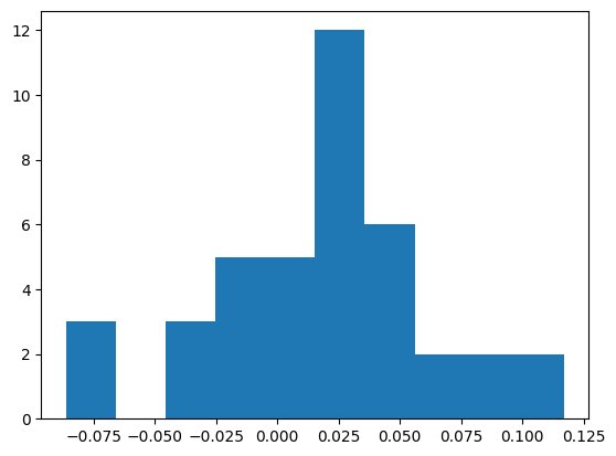

Compared to FFNs with Classification, for regression, we used MSE loss, keeping all else the same (code wise). While making predictions, we just used the outputs of the model as is.